Screen, then optimise: a reactor with a heat-release limit

A pilot reactor makes a product whose yield should be as high as possible, while its impurity must stay below 2.0%. Six factors might matter. The reactor’s cooling jacket removes heat at a limited rate, which rules out running hot with a high catalyst loading.

The study uses 36 runs in three stages:

1. Screen the six factors with a 17-run definitive screening design and keep the ones that matter.

2. Design a 16-run experiment in those factors that respects the heat limit, choosing between D-, I- and G-optimal designs by how well each one predicts over the allowed region.

3. Optimise both responses inside the limit, then confirm the recommended settings with three runs.

A simulator stands in for the reactor. Its equations are in the next cell; the analysis only sees the simulated measurements, and the last section compares the answer with the simulator’s true optimum.

Functions used. generate_design builds every design here, analyze_omars selects the screening model, evaluate_design compares designs over the constrained region, analyze_experiment fits the response surfaces and tests the confirmation runs, and optimize_responses finds the best settings inside the region.

import matplotlib.pyplot as plt
import numpy as np
import pandas as pd

from process_improve.experiments import (
    Constraint,
    DesignRegion,
    Factor,
    analyze_experiment,
    analyze_omars,
    evaluate_design,
    generate_design,
    optimize_responses,
)
from process_improve.experiments.optimization import evaluate_model

The simulated reactor

The true models are written in coded units, where each factor runs from -1 at its low setting to +1 at its high setting. Only temperature T, reaction time t and catalyst loading C affect the responses; pressure P, stirrer speed S and feed ratio R do not. The terms are named the way analyze_experiment names its coefficients, so the same table can be handed to the optimiser in the last section.

factors = [
    Factor(name="T", low=150, high=200, units="degC"),  # temperature
    Factor(name="t", low=10, high=40, units="min"),  # reaction time
    Factor(name="C", low=0.5, high=2.0, units="mol%"),  # catalyst loading
    Factor(name="P", low=2, high=10, units="bar"),  # pressure
    Factor(name="S", low=300, high=900, units="rpm"),  # stirrer speed
    Factor(name="R", low=1.0, high=1.5),  # feed molar ratio
]
RANGES = {f.name: (f.low, f.high) for f in factors}

TRUE_MODELS = {
    "yield": {"Intercept": 70, "T": 6, "t": 4, "C": 5, "T:C": 2.5, "I(T ** 2)": -3, "I(t ** 2)": -2, "I(C ** 2)": -1.5},
    "impurity": {"Intercept": 1.6, "T": 0.2, "t": 0.5, "C": 0.1, "I(t ** 2)": 0.3},
}
NOISE_SD = {"yield": 0.5, "impurity": 0.05}


def to_coded(settings: pd.DataFrame) -> pd.DataFrame:
    """Map actual settings to coded units: -1 at each factor's low setting, +1 at its high."""
    return pd.DataFrame(
        {
            name: (settings[name] - (lo + hi) / 2) / ((hi - lo) / 2)
            for name, (lo, hi) in RANGES.items()
            if name in settings
        }
    )


def true_response(settings: pd.DataFrame) -> pd.DataFrame:
    """Noise-free responses: each term is evaluated on the coded settings (``T:C`` is a product, ``I(T ** 2)`` a square)."""
    x = to_coded(settings)

    def term(name: str) -> pd.Series | float:
        return 1.0 if name == "Intercept" else x.eval(name.replace("I(", "(").replace(":", "*"))

    return pd.DataFrame(
        {response: sum(b * term(name) for name, b in model.items()) for response, model in TRUE_MODELS.items()},
        index=settings.index,
    )


rng = np.random.default_rng(2026)


def run_reactor(settings: pd.DataFrame) -> pd.DataFrame:
    """One measurement of each response per row of settings (actual units)."""
    noise = pd.DataFrame({r: rng.normal(0, sd, len(settings)) for r, sd in NOISE_SD.items()}, index=settings.index)
    return true_response(settings) + noise

1. Screen six factors in 17 runs

A definitive screening design (DSD) runs each factor at three levels, and every main-effect column is orthogonal to every two-factor interaction and quadratic column, so each main effect is estimated free of the second-order effects. The smallest DSD for six factors has 13 runs. Asking for 17 runs builds the design from a larger conference matrix: its two unused columns, the fake factors, carry no factor and leave degrees of freedom for estimating the noise.

screen = generate_design(factors, "dsd", budget=17, random_state=1)
print(
    f"{screen.n_runs} runs; conference matrix of order {screen.metadata['conference_order']}, "
    f"{screen.metadata['fake_factors']} fake factors"
)

# The defining property: every main-effect column is orthogonal to every second-order column.
names = [f.name for f in factors]
x = screen.design[names].to_numpy(dtype=float)
second_order = np.column_stack([x[:, i] * x[:, j] for i in range(6) for j in range(i, 6)])
print("largest |main effect . second-order column|:", np.abs(x.T @ second_order).max())
screen.design_actual.head()

17 runs; conference matrix of order 8, 2 fake factors
largest |main effect . second-order column|: 0.0

	RunOrder	T	t	C	P	S	R
1	1	150.0	25.0	2.00	10.0	300.0	1.5
2	2	200.0	40.0	1.25	2.0	300.0	1.5
3	3	200.0	10.0	2.00	2.0	900.0	1.5
4	4	200.0	10.0	0.50	10.0	300.0	1.5
5	5	150.0	40.0	2.00	2.0	900.0	1.0

analyze_omars selects a model from the screening data in two stages (Jones and Nachtsheim, 2017). Because the main effects are orthogonal to everything else, they are tested first, against an error estimate that the fake factors make possible; the inactive main effects are then pooled into that estimate. The second-order terms are searched next, among the active factors only: with strong heredity, a quadratic or interaction term can enter only if its factors are active.

screen_obs = run_reactor(screen.design_actual)
selected = analyze_omars(
    screen.design[names], screen_obs["yield"], quadratic_heredity="strong", interaction_heredity="strong"
)
print(f"error degrees of freedom: {selected.initial_error_df} before pooling, {selected.updated_error_df} after")
print("main-effect p-values:", {name: round(p, 4) for name, p in selected.main_effect_p_values.items()})
print("active main effects :", selected.active_main_effects)
print("second-order terms  :", selected.active_quadratics + selected.active_interactions)

error degrees of freedom: 2 before pooling, 5 after
main-effect p-values: {'T': 0.0003, 't': 0.0007, 'C': 0.0005, 'P': 0.6809, 'S': 0.8984, 'R': 0.9749}
active main effects : ['T', 't', 'C']
second-order terms  : ['T^2', 't^2', 'C^2', 'T:C']

Temperature, time and catalyst loading are active; pressure, stirrer speed and feed ratio are not, so the next stage holds them at convenient settings. The yield surface is curved in the active factors, so the next design must support the full quadratic model in T, t and C: 10 coefficients.

2. A design that respects the heat limit

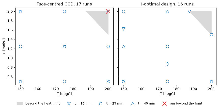
The screening runs were made in a laboratory reactor. In the pilot reactor the heat released must stay within the jacket’s cooling capacity, which in these units is \(0.04\,T + C \le 9.5\): at 200 degC the catalyst loading cannot exceed 1.5 mol%. A face-centred central composite design (CCD) keeps every run inside the factor ranges, but two of its cube corners lie beyond the limit.

active = factors[:3]
heat_limit = Constraint(expression="0.04*T + C <= 9.5")


def heat(settings: pd.DataFrame) -> pd.Series:
    """Heat released, in the units of the limit."""
    return 0.04 * settings["T"] + settings["C"]


def shade_beyond_limit(ax: plt.Axes, **style: object) -> None:
    """Shade the corner of the T-C plane where 0.04 T + C > 9.5 (from T = 187.5 degC at C = 2.0)."""
    T_edge = np.array([187.5, 200.0])
    ax.fill_between(T_edge, 9.5 - 0.04 * T_edge, 2.0, **style)


ccd = generate_design(active, "ccd", alpha="face_centered", n_center_points=3, random_state=1)
print(f"face-centred CCD: {(heat(ccd.design_actual) > 9.5).sum()} of {ccd.n_runs} runs exceed the heat limit")
print(
    f"screening DSD   : {(heat(screen.design_actual) > 9.5).sum()} of {screen.n_runs} runs exceed it (laboratory scale)"
)

face-centred CCD: 2 of 17 runs exceed the heat limit
screening DSD   : 3 of 17 runs exceed it (laboratory scale)

An optimal design is built for a stated model inside a stated region, so the heat limit is part of the problem rather than a repair afterwards. Three 16-run designs are built for the full quadratic model, each by a different criterion. The prediction variance at a point is the variance of the predicted response there, in units of the noise variance:

• D-optimal makes the joint confidence region of the 10 coefficients as small as possible (reported as D-efficiency, higher is better).

• I-optimal makes the prediction variance averaged over the region as small as possible (APV, lower is better).

• G-optimal makes the largest prediction variance in the region as small as possible (reported as G-efficiency, 100% times the number of coefficients over the runs times that maximum; higher is better).

evaluate_design judges each design over the constrained region it was built in, which it reads from the design’s metadata.

designs, rows, curves = {}, {}, {}
for criterion in ("d_optimal", "i_optimal", "g_optimal"):
    design = generate_design(
        active, criterion, budget=16, model_type="quadratic", constraints=[heat_limit], random_state=1
    )
    quality = evaluate_design(
        design,
        model="quadratic",
        metric=["d_efficiency", "average_prediction_variance", "g_efficiency", "fds"],
        fds_resolution=101,
    )
    designs[criterion] = design
    curves[criterion] = quality["fds"]["curve"]
    rows[criterion] = {
        "D-efficiency": quality["d_efficiency"],
        "APV": quality["average_prediction_variance"],
        "max PV": quality["fds"]["max_prediction_variance"],
        "G-efficiency": quality["g_efficiency"],
        "runs on the limit": int(np.isclose(heat(design.design_actual), 9.5).sum()),
    }
pd.DataFrame.from_dict(rows, orient="index").round(3)

	D-efficiency	APV	max PV	G-efficiency	runs on the limit
d_optimal	43.224	0.523	0.965	64.792	4
i_optimal	39.011	0.347	1.132	55.201	3
g_optimal	40.719	0.506	0.775	80.678	3

Each design is best on the criterion it was built for. The fraction of design space (FDS) plot shows more than the average and the maximum: for each design it gives the fraction of the region in which the prediction variance is at or below a given value.

labels = {"d_optimal": "D-optimal", "i_optimal": "I-optimal", "g_optimal": "G-optimal"}
fig, ax = plt.subplots(figsize=(6, 4))
for criterion, curve in curves.items():
    ax.plot(curve["fraction"], curve["prediction_variance"], label=labels[criterion])
ax.set_xlabel("Fraction of the region")
ax.set_ylabel("Prediction variance / noise variance")
ax.set_title("Fraction of design space, inside the heat limit")
ax.legend()
fig.tight_layout()

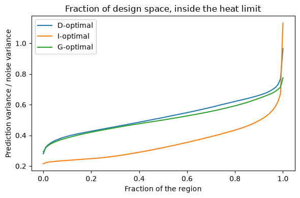
The optimiser will search the whole region for the best settings, so the average prediction variance matters most here, and the I-optimal design is used. Its FDS curve is the lowest over most of the region; the G-optimal design gives that up for a smaller maximum.

The plot below shows the face-centred CCD and the I-optimal design in the temperature-catalyst plane. The CCD’s two runs beyond the limit are crossed out; the I-optimal design instead places runs on the limit itself, the boundary on which the optimum is found in the next section.

stage2 = designs["i_optimal"]
fig, axes = plt.subplots(1, 2, figsize=(9, 4.4), sharey=True)
for ax, (title, design) in zip(
    axes, [("Face-centred CCD, 17 runs", ccd), ("I-optimal design, 16 runs", stage2)], strict=True
):
    runs = design.design_actual
    shade_beyond_limit(ax, color="0.85", label="beyond the heat limit")
    for minutes, marker in [(10, "v"), (25, "o"), (40, "^")]:
        at = runs[np.isclose(runs["t"], minutes)]
        ax.scatter(at["T"], at["C"], marker=marker, s=70, facecolor="white", edgecolor="C0", label=f"t = {minutes} min")
    beyond = runs[heat(runs) > 9.5]
    ax.scatter(beyond["T"], beyond["C"], marker="x", s=130, color="C3", label="run beyond the limit")
    ax.set_title(title)
    ax.set_xlabel("T [degC]")
    ax.set_xlim(147, 203)
    ax.set_ylim(0.42, 2.08)
axes[0].set_ylabel("C [mol%]")
fig.legend(*axes[0].get_legend_handles_labels(), loc="lower center", ncol=5, frameon=False, fontsize=9)
fig.tight_layout(rect=(0, 0.07, 1, 1))

3. Fit, optimise and confirm

The reactor is run at the 16 I-optimal settings and a full quadratic model is fitted to each response, in coded units.

stage2_obs = run_reactor(stage2.design_actual)
fits, coefficients = [], {}
for response in ("yield", "impurity"):
    data = stage2.design[["T", "t", "C"]].assign(**{response: stage2_obs[response].to_numpy()})
    fit = analyze_experiment(data, response_column=response, model="quadratic", analysis_type="coefficients")
    fits.append({"response_name": response, "factor_names": ["T", "t", "C"], "coefficients": fit["coefficients"]})
    coefficients[response] = {row["term"]: row["coefficient"] for row in fit["coefficients"]}
    print(f"{response:8s}: R2 = {fit['model_summary']['r_squared']:.3f}")
pd.DataFrame(coefficients).round(3)

yield   : R2 = 0.998
impurity: R2 = 0.995

	yield	impurity
Intercept	69.841	1.614
T	5.746	0.175
t	3.959	0.517
C	4.755	0.084
T:t	0.178	0.014
T:C	2.788	-0.005
t:C	0.121	0.039
I(T ** 2)	-2.481	-0.041
I(t ** 2)	-1.648	0.311
I(C ** 2)	-1.707	-0.005

Two goals are combined with desirability functions, each mapping a response onto a 0-to-1 scale:

• yield: 0 at 70% or below, rising linearly to 1 at 80% or above;

• impurity: 1 at 1.6% or below, falling linearly to 0 at 2.0%, the rejection limit.

The composite desirability is their geometric mean, so a setting that breaks either limit scores 0. The desirability function below writes out the same calculation, for the plots and the final comparison. Passing the design’s region makes the optimiser keep to the heat limit.

goals = [
    {"response": "yield", "goal": "maximize", "low": 70, "high": 80},
    {"response": "impurity", "goal": "minimize", "low": 1.6, "high": 2.0},
]


def desirability(responses: pd.DataFrame) -> pd.DataFrame:
    """Score the two goals above as linear ramps and combine them by their geometric mean."""
    d = pd.DataFrame(
        {
            "yield": ((responses["yield"] - 70) / (80 - 70)).clip(0, 1),
            "impurity": ((2.0 - responses["impurity"]) / (2.0 - 1.6)).clip(0, 1),
        }
    )
    d["composite"] = np.sqrt(d["yield"] * d["impurity"])
    return d


ranges = {f.name: {"low": f.low, "high": f.high} for f in active}
region = DesignRegion.from_dict(stage2.metadata["region"])
best = optimize_responses(fits, goals, factor_ranges=ranges, region=region)["desirability"]

optimum = pd.DataFrame([best["optimal_actual"]])
print("settings :", {name: round(float(value), 2) for name, value in best["optimal_actual"].items()})
print("predicted:", {name: round(value, 3) for name, value in best["predicted_responses"].items()})
print(f"composite desirability {best['composite_desirability']:.3f}; inside the region: {best['within_region']}")
print(f"heat at the optimum: {heat(optimum).iloc[0]:.2f} (limit 9.5)")

settings : {'T': 190.06, 't': 20.39, 'C': 1.9}
predicted: {'yield': 75.249, 'impurity': 1.628}
composite desirability 0.699; inside the region: True
heat at the optimum: 9.50 (limit 9.5)

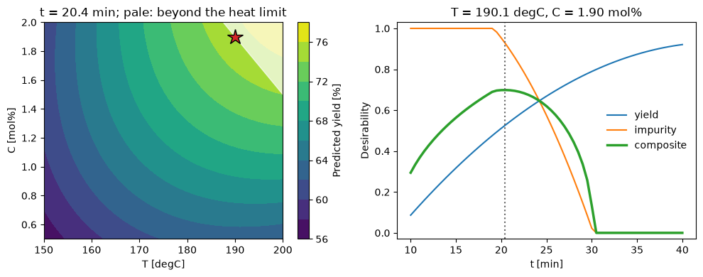
The two panels below explain the recommendation. On the left, the fitted yield at the recommended reaction time rises towards high temperature and high catalyst loading, so the best settings sit on the heat limit. On the right, a longer reaction time raises the yield but also the impurity, and the composite desirability peaks where the two balance.

def predict(settings: pd.DataFrame) -> pd.DataFrame:
    """Fitted responses at settings in actual units (the models were fitted in coded units)."""
    points = to_coded(settings).to_dict("records")
    return pd.DataFrame(
        {
            fit["response_name"]: [evaluate_model(fit["coefficients"], ["T", "t", "C"], p) for p in points]
            for fit in fits
        }
    )


T_axis, C_axis = np.meshgrid(np.linspace(150, 200, 51), np.linspace(0.5, 2.0, 51))
plane = pd.DataFrame({"T": T_axis.ravel(), "t": optimum["t"].iloc[0], "C": C_axis.ravel()})
times = pd.DataFrame({"T": optimum["T"].iloc[0], "t": np.linspace(10, 40, 61), "C": optimum["C"].iloc[0]})
along_t = desirability(predict(times))

fig, (left, right) = plt.subplots(1, 2, figsize=(10, 4))
filled = left.contourf(T_axis, C_axis, predict(plane)["yield"].to_numpy().reshape(T_axis.shape), levels=12)
fig.colorbar(filled, ax=left, label="Predicted yield [%]")
shade_beyond_limit(left, color="white", alpha=0.7)
left.plot(optimum["T"], optimum["C"], marker="*", ms=16, color="C3", markeredgecolor="black")
left.set(xlabel="T [degC]", ylabel="C [mol%]", title=f"t = {optimum['t'].iloc[0]:.1f} min; pale: beyond the heat limit")

for column, label in [("yield", "yield"), ("impurity", "impurity"), ("composite", "composite")]:
    right.plot(times["t"], along_t[column], label=label, lw=2.5 if column == "composite" else 1.5)
right.axvline(optimum["t"].iloc[0], color="0.4", ls=":")
right.set(xlabel="t [min]", ylabel="Desirability", ylim=(-0.03, 1.03))
right.set_title(f"T = {optimum['T'].iloc[0]:.1f} degC, C = {optimum['C'].iloc[0]:.2f} mol%")
right.legend(frameon=False)
fig.tight_layout()

Three confirmation runs at the recommended settings test whether the models predict well where they will be used. Each observation is compared with the 95% prediction interval for a single new run.

confirm = run_reactor(pd.concat([optimum] * 3, ignore_index=True))
coded_point = pd.DataFrame([best["optimal_coded"]] * 3)
rows = []
for response in ("yield", "impurity"):
    data = stage2.design[["T", "t", "C"]].assign(**{response: stage2_obs[response].to_numpy()})
    check = analyze_experiment(
        data,
        response_column=response,
        model="quadratic",
        analysis_type="confirmation_test",
        new_points=coded_point,
        observed_at_new=confirm[response].tolist(),
    )["confirmation_test"]
    rows += [{"response": response, **run} for run in check["results"]]
pd.DataFrame(rows).round(3)

	response	observed	predicted	pi_low	pi_high	within_PI
0	yield	75.312	75.249	73.646	76.852	True
1	yield	75.737	75.249	73.646	76.852	True
2	yield	75.000	75.249	73.646	76.852	True
3	impurity	1.690	1.628	1.474	1.782	True
4	impurity	1.595	1.628	1.474	1.782	True
5	impurity	1.647	1.628	1.474	1.782	True

How close is the answer?

The simulator’s own models, given to the same optimiser with the same goals and region, give the settings the study was looking for. Both rows below are scored on the true responses.

true_fits = [
    {
        "response_name": response,
        "factor_names": ["T", "t", "C"],
        "coefficients": [{"term": term, "coefficient": value} for term, value in model.items()],
    }
    for response, model in TRUE_MODELS.items()
]
truth = optimize_responses(true_fits, goals, factor_ranges=ranges, region=region)["desirability"]

settings = pd.concat([optimum, pd.DataFrame([truth["optimal_actual"]])], ignore_index=True)
responses = true_response(settings)
comparison = pd.concat(
    [settings, heat(settings).rename("heat"), responses, desirability(responses)["composite"]], axis=1
)
comparison.index = ["found", "true optimum"]
print(
    f"the settings found reach {comparison['composite'].iloc[0] / comparison['composite'].iloc[1]:.0%} "
    "of the best composite desirability"
)
comparison.round(3)

the settings found reach 99% of the best composite desirability

	T	t	C	heat	yield	impurity	composite
found	190.056	20.394	1.898	9.5	75.608	1.682	0.668
true optimum	187.554	20.274	1.998	9.5	75.544	1.672	0.674

Summary

• A 17-run DSD with two fake factors picked out the three active factors and the curvature in them. Its main effects are free of every second-order effect, and the fake factors supplied the error estimate the analysis needs.

• The heat limit was part of the second design rather than a repair to it. D-, I- and G-optimal designs were compared on prediction variance over the constrained region, and the I-optimal design, lowest on average, was used.

• The optimum lies on the heat limit, the confirmation runs fall inside their prediction intervals, and the settings found come close to the best the true process allows.

Reference. Jones, B. and Nachtsheim, C. J. (2017). Effective design-based model selection for definitive screening designs. Technometrics, 59(3), 319-329.