Regressing cheddar taste on chemical composition

The cheddar dataset records a panel-tasting score for 30 samples of mature cheddar alongside three chemical measurements that vary with maturation: free acetic acid concentration, hydrogen sulfide, and lactic acid. The question is the standard regression question: how much of the variation in taste can the chemistry explain, and which of the three predictors carries the most weight?

Data. cheddar-cheese.csv from openmv.net. 30 rows, five columns: Case (a sample identifier) and the four numeric variables Acetic, H2S, Lactic, Taste.

What we do. Fit simple linear regression of taste on hydrogen sulfide on its own, then a multiple linear regression on all three predictors, read the coefficient table, and check the residual diagnostics that come with the OLS estimator.

Adapted from the Least squares modelling chapter of the Process Improvement using Data book (CC BY-SA 4.0).

import matplotlib.pyplot as plt
import numpy as np
import pandas as pd
from scipy import stats

from process_improve.regression.methods import OLS

Load the data

The first column is a sample identifier (Case); the next four are the numeric variables we will model. We strip any whitespace from column names so case-insensitive lookups in the next cell are robust to small naming differences between revisions of the dataset.

cheddar = pd.read_csv("https://openmv.net/file/cheddar-cheese.csv")
cheddar.columns = [c.strip() for c in cheddar.columns]
print(f"Shape: {cheddar.shape}")
print(f"Columns: {list(cheddar.columns)}")
cheddar.head()

Shape: (30, 5)
Columns: ['Case', 'Acetic', 'H2S', 'Lactic', 'Taste']

	Case	Acetic	H2S	Lactic	Taste
0	1	4.543	3.135	0.86	12.3
1	2	5.159	5.043	1.53	20.9
2	3	5.366	5.438	1.57	39.0
3	4	5.759	7.496	1.81	47.9
4	5	4.663	3.807	0.99	5.6

# Identify columns case-insensitively so the notebook is robust to small
# naming differences between revisions of the dataset.
cols = {c.lower(): c for c in cheddar.columns}
y_col = cols["taste"]
h2s_col = cols["h2s"]
predictor_cols = [cols["acetic"], cols["h2s"], cols["lactic"]]
y = cheddar[y_col].astype(float)
print(f"Response: {y_col}; Predictors: {predictor_cols}")

Response: Taste; Predictors: ['Acetic', 'H2S', 'Lactic']

Simple linear regression

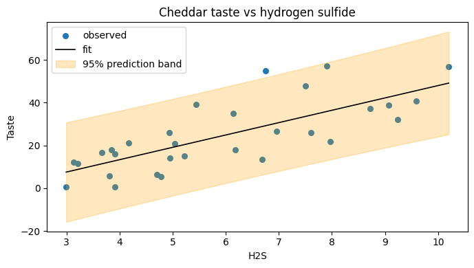
Hydrogen sulfide is the predictor that pid-book singles out as the strongest individual driver. Fitting taste on H2S alone is a useful sanity check; we expect a positive slope (more mature cheese smells stronger and tastes more) and a comfortable signal-to-noise ratio.

model_simple = OLS().fit(cheddar[[h2s_col]], y)
print(
    f"intercept = {model_simple.intercept_:.2f}, "
    f"slope = {model_simple.coefficients_[0]:.2f}, "
    f"R2 = {model_simple.r2_:.3f}"
)
print(f"t-value on slope = {model_simple.t_values_[0]:.2f}, p-value = {model_simple.p_values_[0]:.4f}")

intercept = -9.79, slope = 5.78, R2 = 0.571
t-value on slope = 6.11, p-value = 0.0000

# Scatter plot with fitted line and 95 percent prediction interval band.
x_grid = model_simple.pi_range_[:, 0]
lo = model_simple.pi_range_[:, 1]
hi = model_simple.pi_range_[:, 2]
y_hat = model_simple.intercept_ + model_simple.coefficients_[0] * x_grid

_fig, ax = plt.subplots(figsize=(7, 4))
ax.scatter(cheddar[h2s_col], y, s=30, color="#1f77b4", label="observed")
ax.plot(x_grid, y_hat, color="k", linewidth=1.2, label="fit")
ax.fill_between(x_grid, lo, hi, color="orange", alpha=0.25, label="95% prediction band")
ax.set_xlabel(h2s_col)
ax.set_ylabel(y_col)
ax.set_title("Cheddar taste vs hydrogen sulfide")
ax.legend(loc="best")
plt.tight_layout()
plt.show()

Multiple linear regression

Adding the other two predictors gives the model a chance to explain more of the variation, but tells us less about which predictor matters most: collinearity between the three chemistry variables means the individual coefficient estimates trade against each other.

model_full = OLS().fit(cheddar[predictor_cols], y)
summary = pd.DataFrame(
    {
        "coefficient": model_full.coefficients_,
        "std_error": model_full.standard_errors_,
        "t_value": model_full.t_values_,
        "p_value": model_full.p_values_,
    },
    index=predictor_cols,
)
summary.loc["(intercept)"] = [
    model_full.intercept_,
    model_full.standard_error_intercept_,
    model_full.t_value_intercept_,
    model_full.p_value_intercept_,
]
print(
    f"R2 = {model_full.r2_:.3f}, adjusted R2 = {model_full.adj_r2_:.3f}, "
    f"F = {model_full.f_statistic_:.2f} (p = {model_full.f_pvalue_:.4f})"
)
summary.round(3)

R2 = 0.652, adjusted R2 = 0.611, F = 16.21 (p = 0.0000)

	coefficient	std_error	t_value	p_value
Acetic	0.315	4.464	0.071	0.944
H2S	3.920	1.248	3.142	0.004
Lactic	19.674	8.647	2.275	0.031
(intercept)	-28.854	19.742	-1.462	0.156

Residual diagnostics

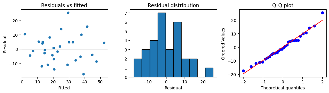
Three quick plots tell you most of what you need to know about whether the linear model is appropriate:

• Residuals vs fitted: should be a horizontal cloud around zero; a U-shape means a curvature term is missing, a fan shape means the variance grows with the fitted value.

• Residual histogram or Q-Q plot: should look approximately normal if you want to trust the t-statistics.

• Residuals vs sample order (if applicable): non-random patterns suggest the rows are not independent.

fitted = model_full.fitted_values_
resid = model_full.residuals_
resid_clean = resid[np.isfinite(resid)]

_fig, axes = plt.subplots(1, 3, figsize=(11, 3.2))
axes[0].scatter(fitted, resid_clean, s=25, color="#1f77b4")
axes[0].axhline(0, color="k", linewidth=0.8)
axes[0].set_xlabel("Fitted")
axes[0].set_ylabel("Residual")
axes[0].set_title("Residuals vs fitted")

axes[1].hist(resid_clean, bins=10, color="#1f77b4", edgecolor="k")
axes[1].set_xlabel("Residual")
axes[1].set_title("Residual distribution")

stats.probplot(resid_clean, dist="norm", plot=axes[2])
axes[2].set_title("Q-Q plot")
plt.tight_layout()
plt.show()

What to try next

• Drop the predictor with the largest p-value and re-fit; compare the coefficient estimates of the two retained predictors. They should change because of the collinearity between the three chemistry variables.

• Try OLS(fit_intercept=False) to see what an origin-passing fit looks like; the diagnostics shift even though the data does not.

• For correlated predictors, switch to PLS to avoid the variance-inflation problem altogether. See the latent-variable case studies for examples.