PCA on NIR tablet spectra

Near-infrared (NIR) spectra are routinely collected for pharmaceutical tablets as an at-line quality check. Each tablet produces a single absorbance spectrum measured at hundreds of wavelengths, so the data matrix is wide (many more variables than samples) and the variables are strongly correlated. PCA is the natural first move: it summarises the dominant patterns in a handful of components and flags individual tablets that do not look like the rest.

Data. tablet-spectra.csv from openmv.net (Kevin Dunn). Each row is one tablet, identified by an alphanumeric code; the remaining 650 columns are absorbance readings at increasing wavelengths.

What we do. Scale the spectra, choose the number of components by cross-validation, look at scores and loadings, monitor the model with SPE and Hotelling’s T squared, and explain a flagged outlier with score contributions.

Adapted from the Principal Component Analysis chapter of the Process Improvement using Data book (CC BY-SA 4.0).

import matplotlib.pyplot as plt
import pandas as pd
import plotly.io as pio

from process_improve.multivariate.methods import PCA, MCUVScaler

# Render Plotly figures as self-contained HTML inside the notebook so nbsphinx
# can embed them in the rendered docs without requiring kaleido.
pio.renderers.default = "notebook_connected"

Load the data

The CSV has no header row. The first column holds the tablet identifier and the remaining columns are the absorbance readings.

spectra = pd.read_csv(
    "https://openmv.net/file/tablet-spectra.csv",
    header=None,
    index_col=0,
)
spectra.index.name = "tablet"
spectra.columns = [f"w{i:03d}" for i in range(spectra.shape[1])]
print(f"Shape: {spectra.shape[0]} tablets x {spectra.shape[1]} wavelengths")
spectra.head()

Shape: 460 tablets x 650 wavelengths

	w000	w001	w002	w003	w004	w005	w006	w007	w008	w009	...	w640	w641	w642	w643	w644	w645	w646	w647	w648	w649
tablet
T001	3.20889	3.20453	3.20592	3.21138	3.22170	3.23109	3.23830	3.24631	3.25275	3.25939	...	4.27016	4.21758	4.66384	4.34843	4.25499	4.10543	4.31009	4.19136	4.09456	4.11117
T002	3.29773	3.29764	3.29745	3.30114	3.31260	3.32110	3.32927	3.34176	3.34129	3.34944	...	4.21997	4.13595	4.12524	4.17672	4.33475	3.92620	4.22542	3.88562	3.93501	4.16061
T003	3.30906	3.30675	3.31150	3.31859	3.32855	3.33675	3.34682	3.35736	3.36218	3.36826	...	4.11644	4.34631	4.13254	4.07010	4.00369	4.06344	3.96726	3.80041	3.86034	4.03759
T004	3.21821	3.21233	3.21379	3.22276	3.23002	3.23915	3.24788	3.25652	3.26485	3.27092	...	4.25797	4.45520	4.82216	4.21016	4.35841	4.12246	4.24843	4.20171	4.18962	4.04324
T005	3.23531	3.23330	3.23519	3.24567	3.25250	3.26385	3.26978	3.28107	3.28788	3.29165	...	4.29922	4.46366	4.37697	4.09199	4.16085	4.64831	4.10806	4.15461	4.15731	4.03757

5 rows × 650 columns

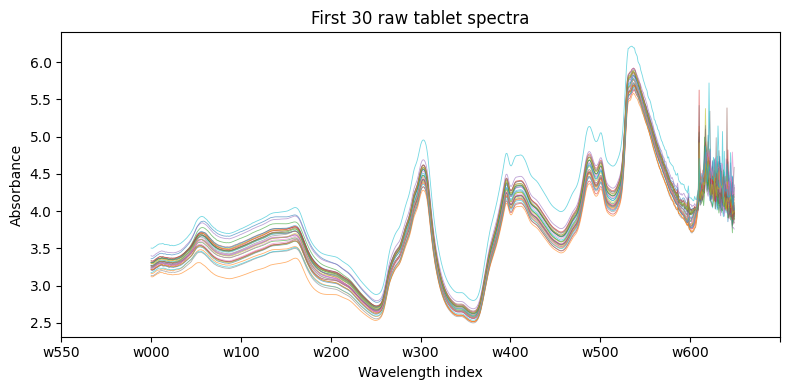
Plotting a handful of raw spectra shows the strong baseline drift and overall correlation that motivate the use of latent variable methods:

fig, ax = plt.subplots(figsize=(8, 4))
spectra.iloc[:30].T.plot(ax=ax, legend=False, linewidth=0.6, alpha=0.6)
ax.set_xlabel("Wavelength index")
ax.set_ylabel("Absorbance")
ax.set_title("First 30 raw tablet spectra")
ax.set_xticks(ax.get_xticks()[::1])
plt.tight_layout()
plt.show()

Preprocess

We mean-centre and unit-variance scale each column with `MCUVScaler <../../../api/multivariate.rst>`__. Without scaling, wavelengths with the largest absolute absorbance would dominate the model purely on account of their range.

scaler = MCUVScaler()
X = scaler.fit_transform(spectra)

Choose the number of components

PCA.select_n_components runs k-fold cross-validation and applies Wold’s criterion to the per-component PRESS values. We cap the search at eight components and use three folds to keep the build time of these docs short; for a real analysis use the defaults.

selection = PCA.select_n_components(X, max_components=8, cv=3)
print(f"Recommended A = {selection.n_components}")
selection.press_ratio.round(3)

Recommended A = 5

n_components
2    0.286
3    0.749
4    0.723
5    0.835
6    0.962
7    0.971
8    0.974
Name: PRESS ratio, dtype: float64

Fit the model

We fit with the recommended number of components, then look at the cumulative R squared to confirm how much of the variability the model captures.

model = PCA(n_components=selection.n_components).fit(X)
model.r2_cumulative_.round(3)

1    0.737
2    0.922
3    0.942
4    0.958
5    0.965
Name: Cumulative R², dtype: float64

Score plot

Each point is one tablet. The ellipse is the 95 percent Hotelling’s T squared limit; tablets outside the ellipse have an unusual combination of PC1 and PC2 scores. Tight clusters within the ellipse suggest that the production lots are repeatable on the dimensions captured by these two components.

model.score_plot()

Loading plot

Loadings tell us which wavelengths drive each component. Wavelengths that sit far from the origin matter most; wavelengths that cluster together are carrying the same information.

model.loading_plot()

SPE and Hotelling’s T squared

SPE measures how well a tablet’s spectrum is explained by the model: a high SPE points to a tablet whose correlation pattern across wavelengths differs from the bulk of the data. T squared measures how far inside the model plane an observation sits: a high T squared is an extreme version of normal behaviour. Tablets that are large on both statistics are the most interesting to investigate.

model.spe_plot()

model.t2_plot()

Outliers

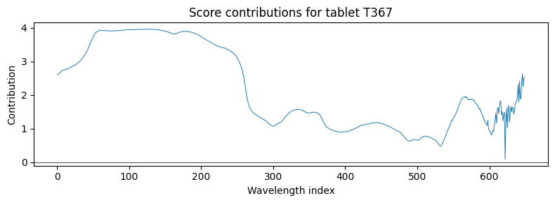
detect_outliers combines the statistical SPE and T squared limits with the robust ESD test. It returns a list of dicts sorted by severity.

outliers = model.detect_outliers(conf_level=0.95)
print(f"{len(outliers)} tablets flagged")
for o in outliers[:5]:
    print(f"  {o['observation']}: {o['outlier_types']} (severity={o['severity']:.2f})")

37 tablets flagged
  T367: ['hotellings_t2'] (severity=2.06)
  T095: ['spe', 'hotellings_t2'] (severity=1.71)
  T385: ['spe', 'hotellings_t2'] (severity=1.57)
  T393: ['hotellings_t2'] (severity=1.54)
  T299: ['spe'] (severity=1.51)

Why is the most extreme tablet unusual?

Score contributions decompose a tablet’s score back into the original wavelength variables. For a flagged tablet we can see which wavelength regions drove it away from the model centre.

worst = outliers[0]["observation"]
scores_worst = model.scores_.loc[worst].values
contrib = model.score_contributions(scores_worst)

fig, ax = plt.subplots(figsize=(8, 3))
ax.plot(range(len(contrib)), contrib.values, linewidth=0.7)
ax.axhline(0, color="k", linewidth=0.5)
ax.set_xlabel("Wavelength index")
ax.set_ylabel("Contribution")
ax.set_title(f"Score contributions for tablet {worst}")
plt.tight_layout()
plt.show()

What to try next

• Use model.predict(X_new) to monitor incoming tablets against the reference model. Compare each new SPE and T squared to model.spe_limit() and model.hotellings_t2_limit().

• If a tablet hardness or assay measurement is available, switch to PLS to relate the spectra to the property of interest.

• Try a robust preprocessing step (Standard Normal Variate, multiplicative scatter correction) before scaling to handle baseline drift more aggressively.

See the PCA user guide for the underlying theory and the `PCA API reference <../../../api/multivariate.rst>`__ for the full method list.