PCA on food texture

A small dataset where five sensory and instrumental measurements are taken on each of 50 pastry samples: oil percentage, density, crispiness, fracture force, and hardness. The variables are correlated and measured on different scales, so PCA on the autoscaled data shows the dominant patterns in two components and lets us identify samples that do not look like the rest of the batch.

Data. food-texture.csv from openmv.net. The first column is a sample identifier; the remaining five are the measurements.

Adapted from the Principal Component Analysis chapter of the Process Improvement using Data book (CC BY-SA 4.0).

import matplotlib.pyplot as plt
import pandas as pd
import plotly.io as pio

from process_improve.multivariate.methods import PCA, MCUVScaler

pio.renderers.default = "notebook_connected"

Load the data

foods = pd.read_csv("https://openmv.net/file/food-texture.csv", index_col=0)
print(f"Shape: {foods.shape[0]} samples x {foods.shape[1]} variables")
foods.head()

Shape: 50 samples x 5 variables

	Oil	Density	Crispy	Fracture	Hardness
B110	16.5	2955	10	23	97
B136	17.7	2660	14	9	139
B171	16.2	2870	12	17	143
B192	16.7	2920	10	31	95
B225	16.3	2975	11	26	143

foods.describe().round(2)

	Oil	Density	Crispy	Fracture	Hardness
count	50.00	50.0	50.00	50.00	50.00
mean	17.20	2857.6	11.52	20.86	128.18
std	1.59	124.5	1.78	5.47	31.13
min	13.70	2570.0	7.00	9.00	63.00
25%	16.30	2772.5	10.00	17.00	107.25
50%	16.90	2867.5	12.00	21.00	126.00
75%	18.10	2945.0	13.00	25.00	143.75
max	21.20	3125.0	15.00	33.00	192.00

The five variables span very different ranges (oil percentage is in the teens, density is in the thousands, the rest are unitless sensory scores). Without scaling, density would dominate the model purely through its variance.

Preprocess and fit

X = MCUVScaler().fit_transform(foods)

selection = PCA.select_n_components(X, max_components=4, cv=5)
print(f"Recommended A = {selection.n_components}")
selection.press_ratio.round(3)

Recommended A = 4

n_components
2    0.338
3    0.649
4    0.362
Name: PRESS ratio, dtype: float64

model = PCA(n_components=max(2, selection.n_components)).fit(X)
model.r2_cumulative_.round(3)

1    0.606
2    0.865
3    0.927
4    0.976
Name: Cumulative R², dtype: float64

Score and loading plots

With only five variables, the loading plot is more useful than for high-dimensional spectra: every loading carries a recognisable label, and we can read directly which sensory and instrumental measurements drive each component.

model.score_plot()

model.loading_plot()

SPE and Hotelling’s T squared

model.spe_plot()

model.t2_plot()

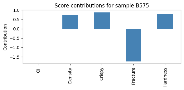
Outlier explanation

Each flagged sample can be explained back in terms of the original five variables with score_contributions.

outliers = model.detect_outliers(conf_level=0.95)
print(f"{len(outliers)} samples flagged")
for o in outliers[:3]:
    print(f"  {o['observation']}: {o['outlier_types']} (severity={o['severity']:.2f})")

1 samples flagged
  B575: ['spe'] (severity=1.77)

if outliers:
    worst = outliers[0]["observation"]
    contrib = model.score_contributions(model.scores_.loc[worst].values)

    fig, ax = plt.subplots(figsize=(6, 3))
    contrib.plot.bar(ax=ax, color="steelblue")
    ax.axhline(0, color="k", linewidth=0.5)
    ax.set_ylabel("Contribution")
    ax.set_title(f"Score contributions for sample {worst}")
    plt.tight_layout()
    plt.show()

What to try next

• The food-texture dataset is small enough that you can recompute everything by hand and check intuition. Try changing the number of components and watch what happens to the score plot, the SPE limit, and the list of flagged samples.

• Compare the loading plot against domain knowledge: do the variables that cluster together in the loading plot also correlate strongly in foods.corr()?

• Once a property like consumer acceptance is added, switch to PLS to relate the texture variables to it.