Factorial DOE: oil-company experiment

Industrial designed experiment from an oil company. Four blend components are varied across 19 runs to improve volumetric heat capacity. Three of the components (A, B, D) are continuous and were varied in coded units; the fourth (C) is a binary factor: present or absent. The aim is to identify which factors and interactions actually drive the response so that future experimentation can focus there.

Data. oil-company-doe.csv from openmv.net. 19 rows, five columns: A, B, C, D, y.

What we do. Run the package’s analyze_experiment with an interactions model, read the coefficient table and ANOVA, build a Pareto plot of standardised effects, and check the residual diagnostics.

Adapted from the Design and analysis of experiments chapter of the Process Improvement using Data book (CC BY-SA 4.0).

import matplotlib.pyplot as plt
import numpy as np
import pandas as pd

from process_improve.experiments.analysis import analyze_experiment

Load and inspect

url = "https://openmv.net/file/oil-company-doe.csv"
doe = pd.read_csv(url, index_col=0)
if doe.shape[1] < 5:
    doe = pd.read_csv(url)
doe.columns = [c.strip() for c in doe.columns]
print(f"Shape: {doe.shape}")
print(f"Columns: {list(doe.columns)}")
doe.head()

Shape: (19, 5)
Columns: ['A', 'B', 'C', 'D', 'y']

	A	B	C	D	y
0	4.38	1.60	No	2.18	28.03
1	6.20	2.26	Yes	2.18	37.25
2	6.20	2.26	Yes	2.18	37.22
3	4.38	2.26	Yes	3.08	37.06
4	6.20	1.60	Yes	3.08	39.23

doe.describe(include="all")

	A	B	C	D	y
count	19.000000	19.000000	19	19.000000	19.000000
unique	NaN	NaN	2	NaN	NaN
top	NaN	NaN	No	NaN	NaN
freq	NaN	NaN	11	NaN	NaN
mean	5.562105	1.970526	NaN	2.685263	33.347895
std	0.795792	0.311582	NaN	0.424884	4.037329
min	4.380000	1.600000	NaN	2.180000	28.030000
25%	4.680000	1.600000	NaN	2.180000	29.565000
50%	6.200000	2.040000	NaN	2.780000	31.710000
75%	6.200000	2.260000	NaN	3.080000	37.140000
max	6.200000	2.260000	NaN	3.080000	39.230000

Fit the interactions model

analyze_experiment accepts a design DataFrame and the name of the response column, builds a formula, fits it via statsmodels, and returns a dictionary keyed by the requested analysis types. With model="interactions" we ask for main effects plus all two-factor interactions; that is 4 + 6 = 10 terms, which fits comfortably in 19 runs.

result = analyze_experiment(
    doe,
    response_column="y",
    model="interactions",
    analysis_type=[
        "coefficients",
        "anova",
        "effects",
        "significance",
        "residual_diagnostics",
    ],
)
ms = result["model_summary"]
print(f"formula     : {ms['formula']}")
print(f"R2          : {ms['r_squared']:.3f}")
print(f"R2 (adj)    : {ms['r_squared_adj']:.3f}")
print(f"R2 (pred)   : {ms['r_squared_pred']:.3f}")
print(f"obs / df_resid: {ms['n_obs']} / {ms['df_residual']}")

formula     : y ~ (A + B + C + D) ** 2
R2          : 0.991
R2 (adj)    : 0.979
R2 (pred)   : 0.963
obs / df_resid: 19 / 8

Coefficient table

Sort by absolute t-value to put the most impactful terms at the top. Coefficients with a small p-value are the ones that the data picks out as important; coefficients whose confidence interval straddles zero are not.

coef_df = pd.DataFrame(result["coefficients"]).set_index("term")
coef_df = coef_df.reindex(coef_df["t_value"].abs().sort_values(ascending=False).index)
coef_df.round(3)

	coefficient	std_error	t_value	p_value	ci_low	ci_high
term
Intercept	61.982	12.449	4.979	0.001	33.274	90.690
B	-116.802	25.774	-4.532	0.002	-176.238	-57.367
A:B	18.047	4.362	4.137	0.003	7.987	28.107
A:D	-10.810	2.930	-3.689	0.006	-17.567	-4.052
D	63.135	19.425	3.250	0.012	18.342	107.929
A	-4.552	2.150	-2.117	0.067	-9.509	0.405
C[T.Yes]	9.418	4.552	2.069	0.072	-1.079	19.914
C[T.Yes]:D	1.207	0.719	1.679	0.132	-0.451	2.866
B:D	3.437	2.236	1.537	0.163	-1.720	8.594
B:C[T.Yes]	-1.741	1.151	-1.512	0.169	-4.395	0.913
A:C[T.Yes]	-0.326	0.424	-0.769	0.464	-1.303	0.651

ANOVA

anova = pd.DataFrame(result["anova_table"]).set_index("source")
anova.round(3)

	df	sum_sq	mean_sq	F	p_value
source
C	1	217.794	None	651.088	0.000
A	1	16.460	None	49.206	0.000
A:C	1	0.198	None	0.591	0.464
B	1	2.502	None	7.479	0.026
B:C	1	0.765	None	2.287	0.169
D	1	9.319	None	27.858	0.001
C:D	1	0.943	None	2.818	0.132
A:B	1	5.725	None	17.114	0.003
A:D	1	4.552	None	13.608	0.006
B:D	1	0.790	None	2.362	0.163
Residual	8	2.676	None	NaN	NaN

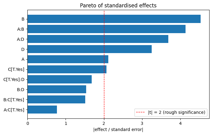
Pareto plot of standardised effects

Dividing each effect estimate by its standard error gives a unitless comparison of how strong each term is relative to the noise. Plotting the absolute values as a horizontal bar chart from largest to smallest is the classical Pareto plot.

effects = pd.Series(result["effects"], dtype=float)
errors = pd.Series(result["effect_std_errors"], dtype=float).reindex(effects.index)
standardised = (effects / errors).abs().sort_values()

_fig, ax = plt.subplots(figsize=(7, 0.35 * max(4, len(standardised)) + 1.0))
ax.barh(standardised.index, standardised.values, color="#1f77b4")
ax.axvline(2, color="r", linestyle="--", linewidth=1, label="|t| = 2 (rough significance)")
ax.set_xlabel("|effect / standard error|")
ax.set_title("Pareto of standardised effects")
ax.legend(loc="best")
plt.tight_layout()
plt.show()

Residual diagnostics

diag = result["residual_diagnostics"]
fitted = np.asarray(diag["fitted_values"], dtype=float)
resid = np.asarray(diag["residuals"], dtype=float)

_fig, axes = plt.subplots(1, 2, figsize=(9, 3.2))
axes[0].scatter(fitted, resid, s=30, color="#1f77b4")
axes[0].axhline(0, color="k", linewidth=0.7)
axes[0].set_xlabel("Fitted")
axes[0].set_ylabel("Residual")
axes[0].set_title("Residuals vs fitted")

axes[1].hist(resid, bins=8, color="#1f77b4", edgecolor="k")
axes[1].set_xlabel("Residual")
axes[1].set_title("Residual distribution")
plt.tight_layout()
plt.show()

print(f"Shapiro-Wilk p-value : {diag['shapiro_wilk']['p_value']:.3f}")
print(f"Durbin-Watson        : {diag['durbin_watson']:.2f}")
print(f"Breusch-Pagan p-value: {diag['breusch_pagan']['p_value']:.3f}")

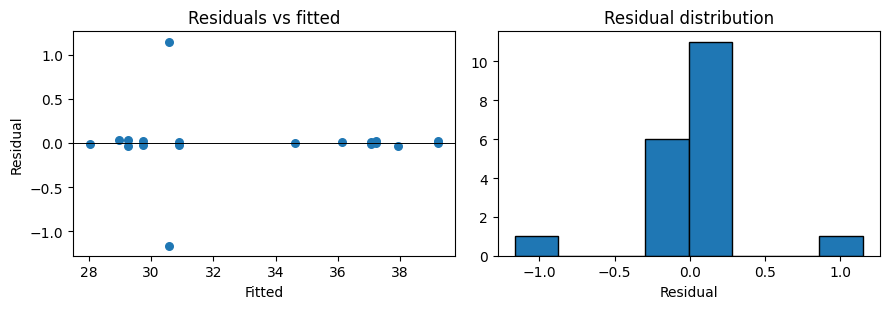
Shapiro-Wilk p-value : 0.000
Durbin-Watson        : 1.52
Breusch-Pagan p-value: 0.050

What to try next

• Drop the terms below the |t| = 2 line and re-fit. The model R squared will go down a touch but the adjusted R squared usually goes up because the noise terms penalise the unadjusted statistic.

• Pass analysis_type="lack_of_fit" to ask whether the residual variation is consistent with pure replication error, which tells you whether a curvature term is missing.

• For follow-up experimentation, the :func:process_improve.experiments.strategy.recommend_strategy function will propose where to run the next batch of experiments given the coefficients you have already estimated.